

调参有啥用?
1、通过尝试不同的参数组合寻找最优组合;
2、也就是说,如果你想要暴富组合,可以通过不断调参,找到暴富因子,如果你想要回撤最小,可以找到稳定增长的参数组合。
3、策略理论应该放在第一,如果策略本身就不行,硬靠调参续命,还不如去买辣条吃。

回测准备
回测标的:btcusdt
回测区间:2019年-至今
回测频度:小时
手续费、滑点:0.050%(交割合约吃单手续费)+0.1%(滑点:指下单的点位和最后成交的点位有差距)
操作方向:只做多,不做空
结论
1、收益率最优参数[10,95](仅针对本次测试组合),综合收益率前十的均线组合,短均线主要聚焦在[10,15,20,25],长均线主要聚焦在[75,80,85,90,95,100];
2、收益率最高的参数组合也只是勉强跑赢基准。


代码
友情提示:行情数据自行准备,涉及行情调取代码不展示
1、使用模块
import pandas as pd
import pymssql
import numpy as np
import datetime
import talib as ta
import matplotlib.pyplot as plt
2、展示格式调整
pd.set_option('expand_frame_repr', False)  # 当列太多时不换行
pd.set_option('display.max_rows', 10000)  # 最多显示多少行
pd.set_option('display.float_format', lambda x: '%.8f' % x) #为了直观的显示数字,不采用科学计数法

#中文
plt.rcParams['font.sans-serif']=['SimHei']
#负号
plt.rcParams['axes.unicode_minus']=False
3、策略函数
def strategy_ma(pdatas,win_short,win_long):
    """
    pdatas:ohlc 格式数据
    win_short:短均线周期
    win_long:长均线周期
    """
    #复制数据,避免在原数据中改动
    datas = pdatas.copy()

    #计算方法:N日移动平均线=N日收市价之和/N
    #长均线计算
    datas['lma'] = ta.MA(datas['close'], timeperiod=win_long)
    #短均线计算
    datas['sma'] = ta.MA(datas['close'], timeperiod=win_short)


    datas['flag'] = 0 # 记录买卖信号
    datas['pos'] = 0 # 记录持仓信号
    pos = 0 # 是否持仓,持多仓:1,不持仓:0,持空仓:-1


    #剔除长均线长度之前的空数据和最后一行数据
    for i in range(max(1,win_long),datas.shape[0] - 1):

        # 当前无仓位,短均线上穿长均线,做多
        if (datas.sma[i-1] < datas.lma[i-1]) and (datas.sma[i] > datas.lma[i]) and pos==0:
            #买卖信号置为1,表明买入
            datas.loc[i,'flag'] = 1
            #买卖信号后一个K线开始持仓,标为1
            datas.loc[i + 1,'pos'] = 1
            pos = 1

        # 当前持仓,死叉,平仓
        elif (datas.sma[i-1] > datas.lma[i-1]) and (datas.sma[i] < datas.lma[i]) and pos==1:
            #买卖信号置为-1,表明卖出
            datas.loc[i,'flag'] = -1
            #买卖信号后一个K线开始持仓,标为0,如果要做空,标志为-1
            datas.loc[i+1 ,'pos'] = 0
            pos = 0


        # 其他情况,保持之前仓位不变
        else:
            datas.loc[i+1,'pos'] = datas.loc[i,'pos']


    #剔除长均线计算之前的空数据,并重置索引,并将原索引删除
    datas = datas.loc[max(0,win_long):,:].reset_index(drop = True)

    return datas
4、资金曲线(与上一版本有区别)
# 计算资金曲线
def equity_curve(data,win_short,win_long,leverage_rate=1, c_rate=1.5 / 1000, min_margin_rate=0.015):
    """
    :param df: 原始数据
    :param win_short: 短均线周期
    :param win_long:长均线周期
    :param leverage_rate:  okex交易所最多提供100倍杠杆,leverage_rate可以在(0, 100]区间选择
    :param c_rate:  手续费,按照吃单万5,滑点千一计算
    :param min_margin_rate:  最低保证金比例
    :return:
    """

    df = strategy_ma(data,win_short,win_long)
    # =====基本参数
    init_cash = 100  # 初始资金
    min_margin = init_cash * leverage_rate * min_margin_rate  # 最低保证金

    # =====根据pos计算资金曲线
    # ===计算涨跌幅
    df['change'] = df['close'].pct_change(1)  # 根据收盘价计算涨跌幅
    df['pct'] = (df['change'].fillna(0) + 1).cumprod() #计算原始收益率
    df['buy_at_open_change'] = df['close'] / df['open'] - 1  # 从今天开盘买入,到今天收盘的涨跌幅,开仓时的计算方法
    df['sell_next_open_change'] = df['open'].shift(-1) / df['close'] - 1  # 从今天收盘到明天开盘的涨跌幅,正常平仓价差计算
    df.at[len(df) - 1, 'sell_next_open_change'] = 0 #最后一根K不处理

    # ===选取开仓、平仓条件
    condition1 = df['pos'] != 0
    condition2 = df['pos'] != df['pos'].shift(1)
    open_pos_condition = condition1 & condition2

    condition1 = df['pos'] != 0
    condition2 = df['pos'] != df['pos'].shift(-1)
    close_pos_condition = condition1 & condition2

    # ===对每次交易进行分组
    df.loc[open_pos_condition, 'start_time'] = df['date']
    df['start_time'].fillna(method='ffill', inplace=True)
    df.loc[df['pos'] == 0, 'start_time'] = pd.NaT

    # ===计算仓位变动
    # 开仓时仓位
    df.loc[open_pos_condition, 'position'] = init_cash * leverage_rate * (1 + df['buy_at_open_change'])

    # 开仓后每天的仓位的变动
    group_num = len(df.groupby('start_time'))


    if group_num > 1:
        #对时间进行分组,与sql不同,其他字段都会依据时间进行分组
        #建仓后的仓位,剔除了开仓
        t = df.groupby('start_time').apply(
            lambda x: x['close'] / x.iloc[0]['close'] * x.iloc[0]['position']
        )
        t = t.reset_index(level=[0])
        df['position'] = t['close']

    elif group_num == 1:
        #按照时间进行分组,但是最后只取其中的收盘跟仓位字段
        t = df.groupby('start_time')[['close', 'position']].apply(
            lambda x: x['close'] / x.iloc[0]['close'] * x.iloc[0]['position'])

        df['position'] = t.T.iloc[:, 0]

    # 每根K线仓位的最大值和最小值,针对最高价和最低价
    df['position_max'] = df['position'] * df['high'] / df['close']
    df['position_min'] = df['position'] * df['low'] / df['close']

    # 平仓时仓位
    df.loc[close_pos_condition, 'position'] *= (1 + df.loc[close_pos_condition, 'sell_next_open_change'])

    # ===计算每天实际持有资金的变化
    # 计算持仓利润
    df['profit'] = (df['position'] - init_cash * leverage_rate) * df['pos']  # 持仓盈利或者损失

    # 计算持仓利润最小值
    df.loc[df['pos'] == 1, 'profit_min'] = (df['position_min'] - init_cash * leverage_rate) * df[
        'pos']  # 最小持仓盈利或者损失
    df.loc[df['pos'] == -1, 'profit_min'] = (df['position_max'] - init_cash * leverage_rate) * df[
        'pos']  # 最小持仓盈利或者损失

    # 计算实际资金量
    df['cash'] = init_cash + df['profit']  # 实际资金
    df['cash'] -= init_cash * leverage_rate * c_rate  # 减去建仓时的手续费,由于前面计算收益率的时候是没有剔除手续费的,所以每个里面剔除即只剔除了一次
    df['cash_min'] = df['cash'] - (df['profit'] - df['profit_min'])  # 实际最小资金
    df.loc[df['cash_min'] < 0, 'cash_min'] = 0  # 如果有小于0,直接设置为0
    df.loc[close_pos_condition, 'cash'] -= df.loc[close_pos_condition, 'position'] * c_rate  # 减去平仓时的手续费
    if len(df[df['cash_min']<= min_margin]['date'].tolist())>0:
        print(df[df['cash_min']<= min_margin]['date'].tolist())


    # ===判断是否会爆仓
    _index = df[df['cash_min'] <= min_margin].index

    if len(_index) > 0:
        print('有爆仓',len(_index))

        df.loc[_index, '强平'] = 1
        df['强平'] = df.groupby('start_time')['强平'].fillna(method='ffill')
        df.loc[(df['强平'] == 1) & (df['强平'].shift(1) != 1), 'cash_强平'] = df['cash_min']  # 此处是有问题的
        df.loc[(df['pos'] != 0) & (df['强平'] == 1), 'cash'] = None
        df['cash'].fillna(value=df['cash_强平'], inplace=True)
        df['cash'] = df.groupby('start_time')['cash'].fillna(method='ffill')
        df.drop(['强平', 'cash_强平'], axis=1, inplace=True)  # 删除不必要的数据

    # ===计算资金曲线
    df['equity_change'] = df['cash'].pct_change()
    df.loc[open_pos_condition, 'equity_change'] = df.loc[open_pos_condition, 'cash'] / init_cash - 1  # 开仓日的收益率
    df['equity_change'].fillna(value=0, inplace=True)
    df['equity_curve'] = (1 + df['equity_change']).cumprod()

    # ===判断资金曲线是否有负值,有的话后面都置成0
    if len(df[df['equity_curve'] < 0]) > 0:
        neg_start = df[df['equity_curve'] < 0].index[0]
        df.loc[neg_start:, 'equity_curve'] = 0
    # ===删除不必要的数据
    df.drop(['change', 'buy_at_open_change', 'sell_next_open_change', 'position', 'position_max',
             'position_min', 'profit', 'profit_min', 'cash', 'cash_min'], axis=1, inplace=True)

    #用于参数回测是区分用
    df['strategy_return%s%s'%(win_short,win_long)] =df['equity_curve']
    #设置时间索引
    df.set_index('date',inplace=True)


    return df
5、穷举调参
#创建空df,含短均线、长均线、收益率三列
single_ids = pd.DataFrame(columns=("win_s","win_l","ret"))
#记录参数集合,画图用
ret_plot=[]
#记录参数、收益率
ret_total=pd.DataFrame()

#短均线,长均线选择数据范围,同时短均线要小于长均线
#短均线选取范围,步长5
for i in range(5,30,5):
    #长均线选取范围,步长5
    for j in range(10,120,5):
        #短均线小于长均线
        if i <j:
            #将参数放到该列表中聚焦
            ret_plot.append('strategy_return%s%s' % (i,j))
            #print(ret_plot)
            print('i:',i,'j:',j)
            #数据回测,思考手续费(资金曲线调整,与上一版本不同)
            result = equity_curve(data,win_short=i,win_long=j)
            #获取最新收益率情况,就是最后一条
            ret = result['equity_curve'].values[-1]
            print(result['equity_curve'].values[-1])
            #收益情况传入df中
            ret_total['strategy_return%s%s' % (i,j)] = result['strategy_return%s%s' % (i,j)]
            #记录短、长均线、收益率结果
            jg_dict = {"win_s":i,"win_l":j,"ret":ret}
            #转df
            jg_dict = pd.DataFrame.from_dict(jg_dict,orient='index')
            #单行df需要转置拼接
            single_ids = single_ids.append(jg_dict.T)
            print(single_ids)
#按照收益率进行降序排列
single_ids.sort_values(by=['ret'],ascending=False,inplace=True)
#重置索引
single_ids.reset_index(inplace=True)# 取收益率前五的进行数据整合
#记录参数集合
ret_plot=[]
#记录参数、收益率
ret_total=pd.DataFrame()
#取收益率前5的参数进行拼接
for i,j in zip(single_ids[:5]['win_s'],single_ids[:5]['win_l']):
#参数取整操作,不取整数,报错,没有细研究,其他代码同上面
i = int(i)
j = int(j)
ret_plot.append('strategy_return%s%s' % (i,j))
#print(ret_plot)
print('i:',i,'j:',j)
result = equity_curve(data,win_short=i,win_long=j)
ret = result['equity_curve'].values[-1]
print(result['equity_curve'].values[-1])
ret_total['strategy_return%s%s' % (i,j)] = result['strategy_return%s%s' % (i,j)]#将基准收益率与策略收益率拼接
result_total = pd.concat([result.pct,ret_total],axis=1)
#去除空行
result_total.dropna(inplace=True)6、画图
#画布大小
plt.figure(figsize = (19,8))
#result_total[ret_plot].plot  #这种写法画布大小无法修改,暂时没解决,有大佬知道,麻烦留言,谢谢!
#不同参数画图
result_total.iloc[:,1].plot(lw=0.8)
result_total.iloc[:,2].plot(lw=0.8)
result_total.iloc[:,3].plot(lw=0.8)
result_total.iloc[:,4].plot(lw=0.8)
result_total.iloc[:,5].plot(lw=0.8)
result_total.pct.plot(c='black',lw=0.8,label='基准')
# plt.title('回测效果')
#添加网格线
plt.grid()
#显示标签
plt.legend()
#画图
plt.show()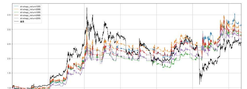

结尾:文章代码仅做交流学习,切勿直接使用进行投资,所产生盈亏概不负责!
文章首发于公众号(CLOUD打怪升级),喜爱可以关注下!

© 版权声明
文章版权归作者所有,未经允许请勿转载。
相关文章


暂无评论...